Criteria for Evaluating Alternative Hypocentres
R J Willemann
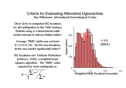
Like many agencies computing hypocentres, the International Seismological Centre may change its location algorithm or travel time model in an attempt to improve hypocentral accuracy. Where so-called ground-truth locations are known, a newly computed epicentre or depth that is closer to ground-truth is certainly superior. For the great majority of events, however, no ground truth location is known. Is there any way to evaluate the quality of new hypocentres for which no ground truth is known?
My answer is that a better hypocentre should fit the data better. Perhaps you agree that this is true in the case of a better travel-time model, but doubt that it is true for a better location algorithm. That case, however, simply emphasizes that importance of measuring the misfit appropriately. For example, if your algorithm assigns different a priori weights to different data, then the misfit measure might include the weights. It turns out, however, that this must be done with some care and that treatment a posteriori weights can be particularly troublesome.
For examples, I'm will use some of the results from a relocation study carried out mainly by Chen Qi-fu of the China Seismological Bureau, who spent most of last year at the ISC as a Royal Society visiting research fellow. Qi-fu is helping the ISC to evaluate the utility of 3-dimensional global tomographic models for routinely locating earthquakes for the ISC Bulletin. His objectives last year were based on simply replacing the Jeffreys-Bullen travel times with various other models. For the relatively few events with good ground truth he obtained the most accurate locations with a block model of Kelli Karason and Rob van der Hilst. I will be using Qi-fu's relocations of about 3800 ISC earthquakes of 1998/January, which includes no ground-truth events.
What I show on this slide is that, at first glance, there appears to be very little improvement in the travel time residuals - the average of the RMS misfits was reduced by just a few per cent. If you study the histogram of RMS residuals you may be able to convince yourself that there is "clear" improvement but even if we managed to show that this change is statistically significant I think that you would agree with me that the improvement is surprisingly small. Now one thing that we have to keep in mind is that the misfit computed by the ISC is a weighted RMS value. The weights are computed using Jeffreys' method of Uniform Reduction, which enabled Jeffreys and Bullen to develop their famous travel time tables.
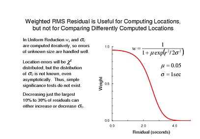
Unlike standard weighted least squares, Uniform Reduction assumes no a priori information about data quality, but instead assigns smaller weights to arrival times with larger residuals. The weights must be computed iteratively, of course, based on the residuals in the previous iteration. There is one free parameter, m, for which the ISC always uses 0.05. The other apparent parameter, s, is actually computed iteratively as well: it is weighted RMS, computed from the residuals and weights of the previous iteration.
This "data dependent" parameter turns out to have some peculiar effects. Suppose, for example, that the original data include some clear outliers, say 10% to 30% of residuals are twice as large as the rest of the data. Suppose, further, that you find some way to bring those in-line with the other data, perhaps they come from stations where inaccurate station corrections were used previously. It is easy to show with some numerical trials that your final estimate of sU is quite likely increase! The reason is that the outliers were previously assigned w = 0 and made no contribution to sU. But after correcting them, the former outliers do contribute to sU and, of course, are as likely to be larger than the other residuals as smaller.
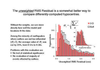
We could try simply ignoring the weights when computing a final misfit value. I am not suggesting abandoning Uniform Reduction - the locations are still computed in the same way with iteratively updated weights and sigma. I'm saying that after we have computed the hypocentres using Uniform Reduction, let's re-calculate the data misfits ignoring the weights. So that's what I've plotted here and, I hope you'll agree, improvement of the residuals as a result of using a 3-D model is much more clear. (As a reminder, I have included the histogram of weighted RMS from the first slide in miniature.)
Now among these unweighted RMS values, the larger ones are quite meaningless: many of the values > 1s are heavily influenced by a few large outliers. Thus, to quantify the improvement I might simply say let's consider all of the events where the unweighted RMS misfit of the original locations was <1s. For these events the new travel time model and relocations cut the average RMS misfit from 0.51s to 0.38s. This is a 25% reduction, which is certainly much better than the reduction of the weighted RMS residual.
Perhaps you are still disappointed. After all, we are switching from a model developed closer to the year when seismometers were invented than to the present. You had hoped, maybe, that the improvement would be expressed not as a percentage reduction but as a factor - 3 times smaller errors, 5 times, who knows, 10 times smaller errors. Perhaps the problem is that we are ignoring exactly the cases where the most improvement was possible: where the residuals were large!
Also, the question of statistical significance has still not been addressed. So these are the two issues I want dig into: statistical significance and a way to include all of the data.
These histograms show the shape of the probability density functions. Perhaps they even look like chi-square distributions to you. Unfortunately, since the data include many outliers, they are not expected to be chi-square and, in fact they do have large deviations from chi-square even if you take account of the number of stations used to compute each hypocentre. Without a good statistical model it is very difficult to state the uncertainties of the means. That is, while we can say that the mean unweighted RMS of Bulletin residuals is 0.51, we cannot say, for example, that it was 0.51 ± 0.03, meaning that we expect it to be between 0.48 and 0.54 in about ten out of twelve months each year.
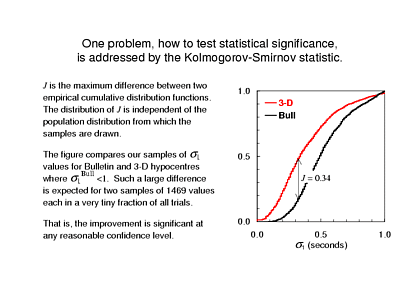
If, instead of plotting the density distributions we plot the cumulative distributions then, perhaps, you will be reminded of a very well-known test of statistical significance. These plots are based on the same data as the histograms, but show the integrals of the density function. If these were two independent samples drawn from the same population, then their cumulative distributions would never differ very much. In fact, they differ by quite a bit: Out of all events that were "not too bad" to begin with, only about 1 in 8 Bulletin hypocentres have an unweighted RMS residual less than 0.3s, but nearly half of the hypocentres computed with Karason and van der Hilst's model fit the data this well.
One standard way of comparing two distributions plotted this way is the Kolmogorov-Smirinov test. Kolmogorov and Smirnov showed how to compute the probability of the CDF's of two samples from the same population differing by any given amount, without making any assumptions about the population distribution. That's exactly what we require here, since we don't know the distribution of residuals.
With samples of more than 1400 values, a difference as large as this is basically impossible for two samples drawn from the same population - the probability of this happening by chance is something like 10-137. So, Qi-fu's relocations of ISC events achieved a better fit to the data with a very high level of confidence.
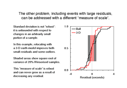
The other problem with the tests that we have looked at so far is treatment of large residuals, which unduly influence the unweighted RMS, or standard deviation. The feature of standard deviation that is causing trouble is that it is not robust. That is, an arbitrarily small fraction of the data - even just one sample - can wreak complete havoc.
Now, what I have shown here is the cumulative distribution function of arrival time residuals for one earthquake. The residuals from the ISC Bulletin are shown in black and the residuals from Qi-fu's relocation are shown in red, and each set looks reasonably well-behaved. The density function is proportional to the slope, so it has a high value near r=0 and smaller values for larger positive or negative residuals - that is, the residuals more or less normally distributed.
In a normal distribution, 68% of the values are within 1 standard deviation of the mean. In this example the standard deviation of Qi-fu's residuals is 0.9s, but 80% of the residuals are within ±0.9s, quite a bit more than 68%. What's gone wrong is that there is one moderately outlying residual of -2.5s, which changes the standard deviation so much that it no longer remotely represents the range over which we find 68% of the values.
Of course if that's what we really wanted we could just compute it: sort the absolute value of residuals, go up to 68% and, bang, that's our measure of how broadly the residuals are distributed. Some people would object that this ignores the other 32% of the data but it doesn't, really, because those other 32 out of every 100 values tell us where to draw the line. Some unknown fraction of the values beyond that are outliers, so we are happy to limit their role computing our statistic in order to make it robust.
Actually, the flaw in the 68th percentile measure is that it doesn't make as much use as it might of small residuals, i.e. the good data. Just as large residuals can be increased without bound and leave the 68th percentile unchanged, so almost all of the small residuals could be reduced to 0, leaving aside the values just below the 68th percentile, and the statistic is unchanged. Thus, a better measure of the scale of the residuals is to set aside some fixed fraction, starting from the largest ones, and then compute the mean square of those that remain. Statisticians call this "trimmed variance". It is no longer an estimate of sample variance, but it is robust and it does take full advantage of all of the "good data", i.e. values within the fraction of all data that we decide to keep.
An alternative to trimming the sample, throwing away some of the data, is to "Winsorise" it, which means to take all of the data that we were about to throw away and instead pretend that they have values equal to the largest ones that we are keeping. It sounds peculiar, but statistics of the Winsorised sample have the same robustness features as those of the trimmed sample, yet for samples without any outliers the Winsorised statistics are somewhat closer to the standard sample statistics.
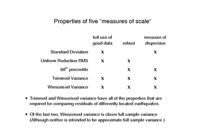
So, I have mentioned five different "measures of scale", and let's review their properties. Standard deviation takes advantage of all good data - the small residuals - but it is not robust because it tries too hard to take advantage of all the data, some of which are outliers. Uniform Reduction also takes advantage of all good data, by assigning them large weights and it achieves robustness by assigning null weights to outliers. Unfortunately it has the flaw I described previously of sometimes getting larger when we reduce some of the residuals. Statisticians refer to a measure of scale that avoids this flaw as "measures of dispersion", so we can say that the Uniform Reduction RMS fails to be a measure of dispersion.
Each of the other measures of scale is robust and a measure of dispersion; in principal we could use any of them compare differently computed hypocentres. But the 68th percentile would fail to show improvement if we only made the good half of the residuals better, so I'm not going to use it. Between the trimmed variance and the Winsorised variance it really doesn't make any difference. Actually, I sort of wish that I had used the trimmed variance because it's easier to describe, but that's not what I did and so, rather than re-computing everything I'm going to show results using the Winsorised variance.
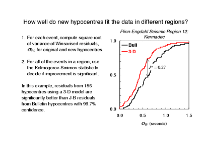
So, we are interested in how well a new travel time model or algorithm works with different subsets of the events. If it was a new algorithm we might be interested in how well it performs when there are only a few stations or when the station distribution is poor. For the example I'm using the model accuracy varies from place to place, so I'm going to look at regional subsets. From the viewpoint of the method it doesn't really matter: somehow the evaluator chooses potentially interesting subsets of the events.
For each event in a subset, I compute the square root of the Winsorised variance of its residuals, i.e. this robust measure of dispersion that I have described. I used the 20% Winsorised sample. This sounds pretty extreme - throwing away the 20% largest values and the 20% smallest leaving me with only 60% of the original sample, but it's what they do in all of the text books on robust statistics, so as I set out across this relatively unfamiliar terrain I'll just follow the convention.
So now I have two numbers in hand for each earthquake: the root Winsorised variance of the Bulletin residuals and of the re-location residuals. I sort each set of numbers, plot the sample CDF's, as shown here, measure the Kolmogorov-Smirnov statistic, and then compute the level of confidence with which I can say that the samples differ. This example is for Flinn-Engdahl region 12 - Kermadec - and the samples differ with more than 99.9% confidence. That is, re-location of Kermadec trench earthquakes using the 3-dimensional model has definitely improved fit to the data.
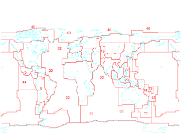
So, I repeat this for the 50 Flinn-Engdahl seismic regions around the world. Actually I do it for 48 regions because Qi-fu's test included no events in two of the regions. Now, if the changes were actually random rather than genuine improvements then I would expect the confidence levels to be uniformly distributed between 0% and 100%. That is, just by chance I would expect 10% - 4 or 5 of 48 regions - to have distributions that apparently differ with more than 90% confidence. If fact it turns out that the difference is significant at the 90% level in 13 of 48 regions, or more than one quarter.
One thing to keep in mind here is that the Komogorov-Smirnov test has relatively "low power". That is, when we control the rate "false positives", the test will produce a large rate of "false negatives". Obviously this is not desirable; it's the price we pay for not knowing the population distribution.
So, in the global map of Flinn-Engdahl regions I have blanked out the identifying numbers in most cases - I left in the numbers for the 13 regions where the distribution of Winsorised RMS is most significantly changed. Many of them are regions with poor station coverage - broad oceans and the southern hemisphere generally. There are exceptions to this characterisation of regions where we were able to improve ISC hypocentres; the Philippines have excellent coverage of course. But regions 11-14 have the most significant improvement of all, and the poor station coverage in this part of the world is notorious, since only Australian and New Zealand stations to their west and south record many events.
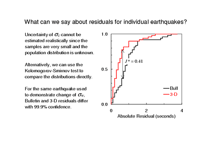
Well, having identified subsets of events where some new hypocentres fit data particularly well, or poorly, we will probably want to take a look at individual earthquakes. We never did solve the problem of estimating uncertainty of our statistics: we can say what the value of Winsorised variance is, but we can't given an uncertainty and then expect some known fraction of the values to fall in that range, say for events next month.
So, we're back to using the relatively low-power Kolmogorov-Smirnov test, this time to compare residuals of individual earthquakes. Since the number of values in each sample can be quite small we're going to suffer from a high rate of false negatives: instances where the test fails to show that the residuals have been improved. We also face the problem that the two sample are not drawn from completely independent populations. The new travel times have, hopefully, corrected a large part of the model error that contributes to the residuals but errors arising from mis-measured time, mis-association of arrivals, and so on are all common to the two samples. So, realistically, we might come to use quite low confidence levels to point us to earthquakes where residuals have changed enough to be interesting.
This example is the same one that I used earlier when I described the Winsorised variance. In this case we don't have to worry about all of those caveats about low power and dependent populations: the change in the residuals is significant at more than the 99% confidence level.
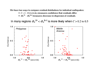
So, we now have two ways to compare the residuals from different hypocentres for an earthquake: the Kolmogorov-Smirnov confidence that the distributions differ and the difference between the root Winsorised variances, for which I cannot estimate an uncertainty (or even a confidence that it is non-null), but which at least does give me an idea of whether the new hypocentre made the residuals better or worse.
OK, two interesting numbers for many examples - let's make a scatter plot and see if there's any relationship between them. Here's what I found: In most of the 13 regions where I previously reckoned that there was a significant change, the difference between the Winsorised variances indicated improvement in almost every case where the Kolmogorov-Smirnov confidence exceeded something like 0.2. I show examples from a couple of the Flinn-Engdahl region here. I think that we're really getting somewhere; we have good evidence that while the residuals do become somewhat more dispersed in some cases, those are just the earthquakes where we didn't change the residual distributions perceptibly anyway.
What's more, we have a general rule that works so well that the exceptions are rare enough that we can think about taking a look at them individually to try and work out what went wrong. If, instead, there were many points in the upper right quarter of these figures then we might be seriously concerned, since there was a good number of earthquakes where we changed the residuals a lot, and they got worse.
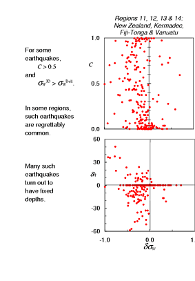
Let's take a closer look at those four southwestern Pacific regions, New Zealand, Kermadec, Tonga-Fiji and Vanuatu, where the change in the distribution of Winsorised variances was most significant. First the moderately good news: the Winsorised variance indicates that we have reduced dispersion of the residuals for 183 out of 242 these earthquakes. The bad news, of course, is that we have increased dispersion of the residuals for the other 59 earthquakes and, more seriously, we have done so while changing the residuals significantly in many cases. That is, there is an uncomfortably large number of earthquakes for which the relocation changed the residuals quite a bit and made them worse!
The most striking thing that I found among earthquakes in these regions is that, with only a few exceptions, the residuals became more dispersed only when the re-location was done with a fixed depth. That is, if the re-location failed to converge with a free depth, the program fixed the earthquake at the depth in the Bulletin hypocentre and tried to converge on a solution that way. That's why there's this concentration of points representing earthquakes for which the Bulletin and 3-D hypocentres have exactly the same depth. It didn't just work out that way; the data were insufficient to tell the depth, so depth in re-location was fixed to the depth in the Bulletin. The fact that the residuals often became more dispersed tells us that, while we don't know the depth, in those cases the 3-D travel time model is not very consistent with the Bulletin depth.
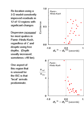
Before I give a summary of the methods that I've talked about, I must describe the results for one of the 13 regions where the Komogorov-Smirnov test indicated a significant change in the distribution of Winsorised variances - region 48, "Pamir - Hindu Kush". For 23 of 25 the test events in this region the Winsorised variance increased: the residuals became more dispersed. What's more, the Kolmogorov-Smirnov test for comparing the residual distributions of individual earthquakes often gave a confidence greater than 0.2. That is, by the criterion that I have become accustomed to indicate significant changes in the residuals, these residuals really did change. And they got worse!
After what I saw in the southwestern Pacific, the first thing I looked for was fixed depths. No joy there: these earthquakes mostly have depths of 100 - 150 km in the Bulletin, and with the 3-D model the hypocentral solutions converged with a free depth again, usually ending up 10 - 20 km deeper, and occasionally >40 km deeper.
This region is extraordinary on several counts, there is no place in the world with crust much thicker than here. For earthquakes at mantle depths thick crust would not ordinarily have much of an effect on the majority of ISC hypocentres, since we think of ourselves as computing teleseismic locations. Many of the earthquakes in this region are located using a proportion of locally recorded times that is unusually large, at least compared to the other 12 regions where residuals changed significantly
Ray paths used in the tomographic inversion are not as dense here as in some other regions, so the model may be less accurate here. Alternatively, perhaps we have not been sufficiently thorough in making use of a realistic 3-D mantle model, but it is not immediately apparent how this could explain why changing from the J.-B. travel times (with no crustal corrections) actually made things worse
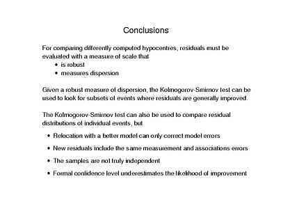
In the last few slides I have started to take a close look at some features of Chen Qi-fu's re-locations using Karason and van der Hilst's tomogrphaphic model. My main point is somewhat more general: that the fit to the data is an important feature of any set of hypocentres, and that a quantitative comparison of how well two sets of hypocentres fit the data can be meaningful. There are a few caveats.
First, the misfit measure must have a couple of properties that, fortunately, statisticians have already described pretty well. One of them, however, is not a property of most misfit measures used in iteratively computing hypocentres.
Second, incomplete knowledge of the population distribution limits our choice of tests for statistical significance. And third, the residuals from two sets of hypocentres computed from the same data are not really independent. Both of these latter two points tend to increase the rate of false negatives. That is, if you put complete faith in the statistical tests, then things are probably better than you think.

